Bayesian Optimisation vs. Input Uncertainty Reduction
This is the work of Juan Ungredda Google Scholar, Student Homepage
Problem Setting
Playing with complex systems in the real world, queing systems, productions lines, traffics lights, can be costly and possibly dangerous. In simulation optimization, we use computer simulations instead as they are faster and less risky. We can then apply automated optimization algorithms to these simualtors to find the best possible settings, then these settings may be used in the real world.
However, simulators must be calibrated to a given scenario, for example I want to simulate a specific set of traffic lights with given layout and traffic flows. This is referred to the problem of input uncertainty. If I use a simulator with input parameers that don’t match the real world scenario, an optimizer will find optimal settings that cannot be applied to the real world.
In this work, we ask the question “What if I could collect simulation calibration input data while I am running my optimizer?”
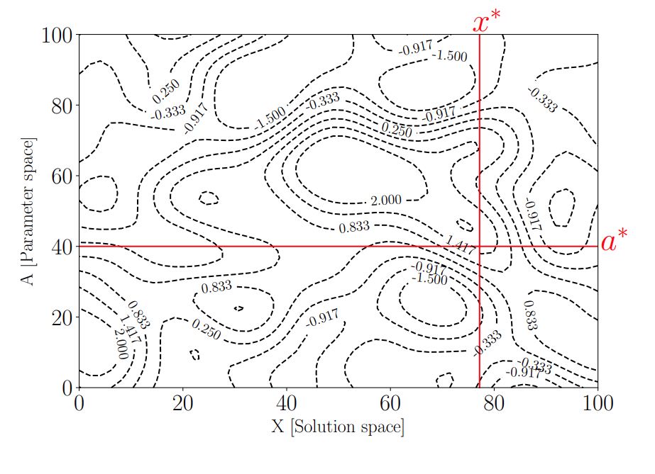
Mathematically, we assume the simulator is a simply an expensive black box function with two arguments \(f(x, a)\), a decision variable to optimize, \(x\), as well as a calbration parameter, \(a\). We want to simultaneously
- collect real world data to tune the callibration parameter \(a\) towards \(a^*\) hence the simulator \(f(x, a)\) is accurate,
- search for the best \(x^*\) that is the best input to the simulator
[x* = argmax f(x, a*)]
For example, if \(x\) and \(a\) are both scalar, \(f(x,a)\) may look as follows
Algorithm Design
We do this by building two models
- a distribution over \(a\)
- a surrogate model of the simulator \(f(x, a)\)
And from these models we design a sequenctial algorithm that decides between collecting more real world data and updating the posterior distributino of \(a\) or instead choosing a simulation point \(y_i = f(x_i, a_i)\). The aalgorithm automatically detemrines the trade off between which type of data to collect and continues until a stopping criteria e.g. given budget has been consumed.
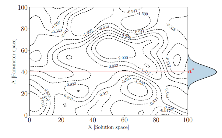
Modelling Input Parameter Values \(a\)
For the \(a\), we collect real world data and we build a posterior distrubtion over values of \(a\) that hopefully converges towards the true \(a^*\) with increasing data. Thus, the problem of simulation optimization becomes one of optimizing the simulator for a range of \(a\) values, some more likely thean others, as shown below by the blue distribution
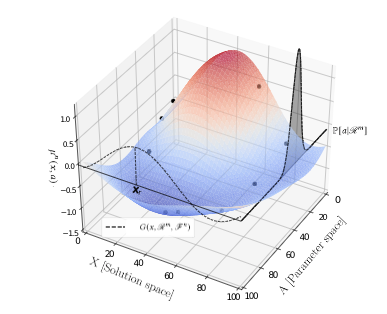
Modelling the Expensive Simulator \(f(x, a)\)
After having evaluated the simulator for at \(n\) points \((x_1, a_1, y_1),....,(x_n, a_n, y_n)\) where \(y_i=f(x_i, a_i)\), this may be used as a dataset to fit a Gaussian Process. See below wheer black points are the simulation evalution points, and the surface shows the GP posterior mean.
Data Collection
We adopt a Bayesian Decision Theoretic formulation in which we can quantify the value of information of collecting data to learn about \(a^*\) as well as or running the simulator \(y=f(x,a)\). At each algorithm iteration, the algorithm simply chooses the action with the highest value.
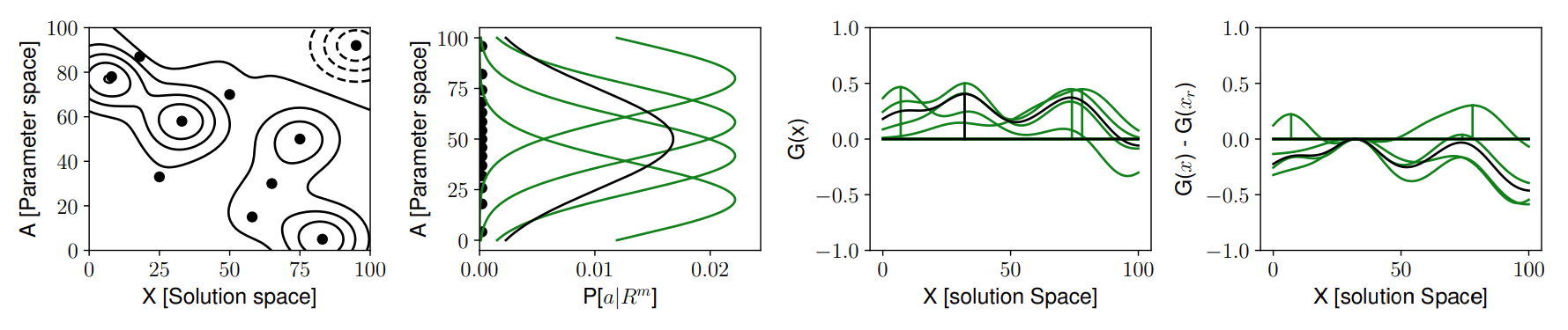
Collecting \(a\) Data
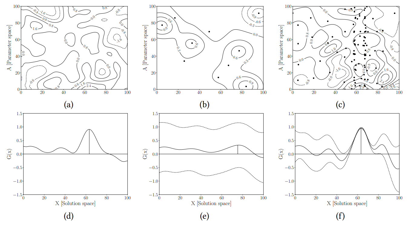
We can collect data to learn more about \(a^*\) by looking at how the distributuion for \(a\) would change, perform one step look ahead. Below, on the left we have the function \(f(x,a)\), next is the current distirbutino of \(P[a]\) in black, and multiple possible future predictive distributions of \(P[a]\) in green. Next is the integrated function
| [\int_a f(x,a)P[a | \text{data}]da] |
for each possible distribution of \(a\) and the peak of each integrated function. Finally, with a little control variate trick, we compute the average of these peaks to quantiy the value of information.
Collecting \(f(x, a)\) Data
We use the algorithm described in this post and provide a TLDR here. We may evaluate the simulator \(f(x, a)\) at a given point \((x, a)\) and update the model, below is the model, black poitns are past data, and the greeen point is a range of possible future \(y\) values at a given \((x, a)\) input. The green line is the one step look ahead integrated function (exactly as with the previous figure). We take the peak of all these realisations of the one-step lookahead integrated functions.
If we collect lots of simulation data
Experiments
See the paper for more details, I’ll be back!