Bayesian Simulation Optimization with Input Uncertainty
In this paper we extend the Expected Improvement (EI) and Knowledge Gradient (KG) BO algorithms to be able to account for optimising a function averaged over one of it inputs, specifially find
[\text{argmax}_{x}\int_a f(x,a) \mathbb{P}[a]da.]
Or Bayesian optimisation with quadrature, one must sequentially choose \((a,x)\) pairs to learn trhe best output integrated over \(a\). This has been been covered by other works, 2013 NeurIPS paper “Multi-Task Bayesian Optimisation” that uses EI and a two-step heuristic to find \((x,a)\), almost identical to this work is a 2018 arxiv paper “Bayesian Optimisation of Expensive Integrands” that uses KG. More recently I stumbled across a 2018 AAAI paper “Alternating Optimisation and Quadrature for Robust Control” that is independent of all the rest and also uses a step heuristic (the paper we present here is 2017).
In the simulation optimisation community (where we work), a user designs a simulator \(f(x,a)\) as a surrogate of the real world where \(x\) are decision variables to be optimised, an \(a\) are unknown simulator settings or parameters. Such a simulator must be callibrated to real world data, set the correct \(a\) value.
For example, to optimise traffic light timings at a given (real world) road intersection, a user may write a simulator of the intersection and the surrounding roads with randomly spawned cars driving around. If the true real arrival rate of cars \(a\) is not known, it must be estiamted which comes with some uncewrtainty and we really learn \(\mathbb{P}[a]\). Given such a simualtor the best one can do is find a single \(x\) that is best across a range of \(a\) values.
As a quick refresher, the Expected Improvement acquisition function asks the questions how much will the observed peak improve and looks like the following
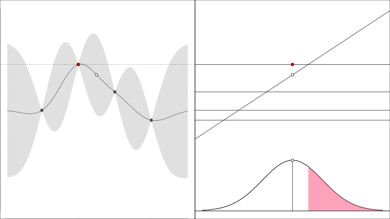
the red point is the height of the largest \(y\) value found so far, if the data is hypothetically augmented with a new point (just to the right of the current best point) then that new point has some chance of being better or worse than the current best in which case there is an improvement, or it may be worse, in which case there is nothing, the expectation of these outcomes quantifies EI(X).
Knowledge Gradient generalises the EI to noisy functions (since comparing raw \(y\) values is somewhat meaningless when they are noisy) and it instead asks the question how does the predicted peak improve:
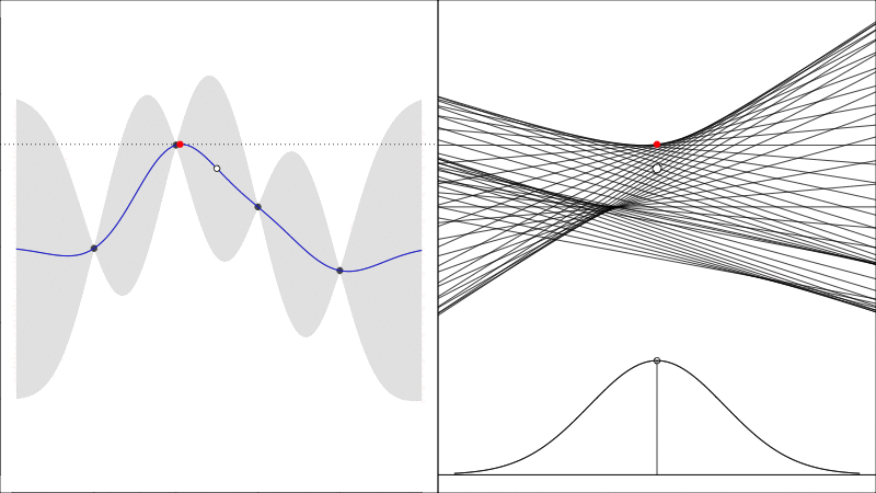
graphically, the average height of the red point in this second plot shows how much it is worth colecting the white data point whose \(y\) value is random.
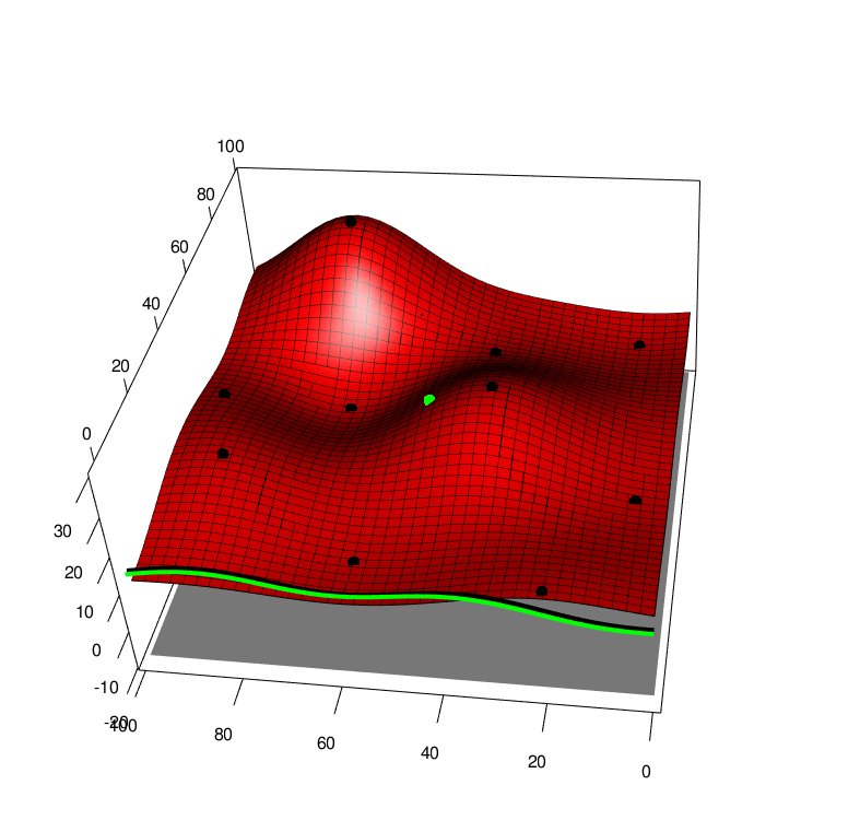
Extending both of these approaches to the case of a function averaged over one of it arguments, we first extend the GP to model function over both arguments \(f(x,a)\sim GP(x,a)\) and this also leads to a GP over the average \(F(x) \sim GP(x)\). By collecting data \((x,a)\) we recieve a new \(y\) value that will affect the predcition of the average \(F(x)\), this can be seen in the following picture, \(x\) is horizontal, \(a\) is depth and \(y\) is height. The black line is the GP averaged over \(a\), and the green line is the GP averaged over \(a\) with one new (random) observation added to the training set. So we can look at the green line and apply Knowledge Gradient or with some approximations expected improvement
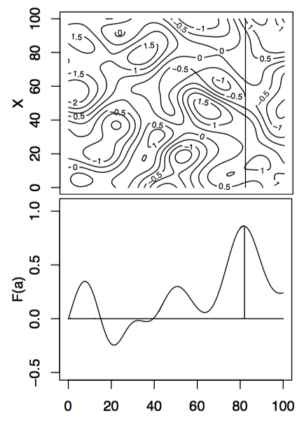
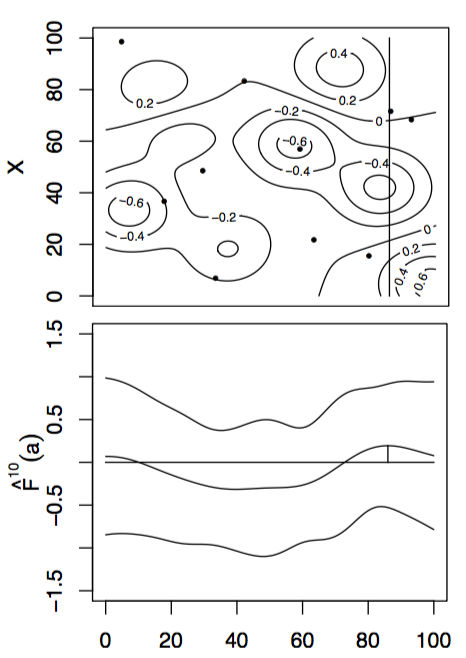
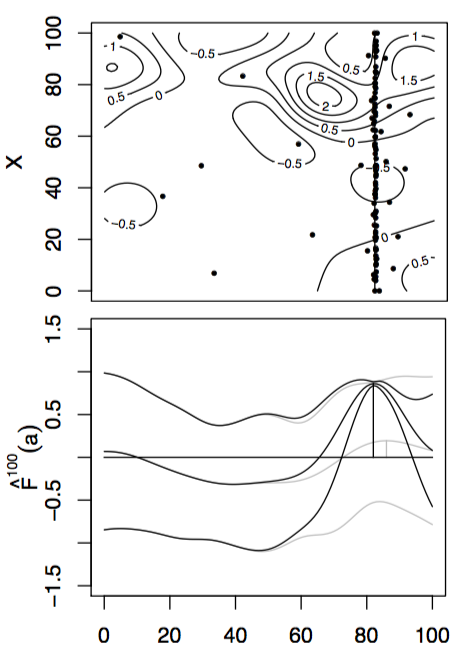
With these modifications, we can apply these new algorithms to some simple test functions, left is the test function, bottom is the function integrated along the viertical axis with the peak shown. Centre is the GP before at the begining with 10 points, right is the GP after 100 points determined by Expected improvement with input uncertainty.
Finally, plotting the opportunity cost between the best possible \(x^*\) and the predicted peak \(x = \text{argmax}_x\int_a \mu(x,a)\mathbb{P}[a]da\) as sampling increases, KG+IU in blue, EI+IU in green and random selected \((x,a)\) in pink.
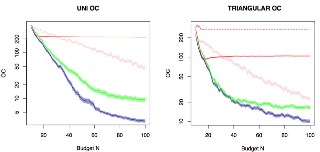
On the left we set \(\mathbb{P}[a] = Uniform(0,100)\) and red is the standard EI applied to the average \(\mathbb{E}[a]=50\) which fails to converge, it is obviously the wrong tool for the job. Right is where \(\mathbb{E}[a]=Triangular(min=0,max=100,peak=100)\) which is a wedge shape distribution and the solid red is the mean \(a = 66.6\) value while dashed red is the mode \(a=100\) value. Again both methods will not converge.