Bayesian Optimization Allowing for Common Random Numbers
This is joint work with Matthias Poloczek from Uber AI and Juergen Branke of Warwick Business School.
Common random numbers (CRN) is a widely used tool in the simulation optimisation, running simulations under different settings however with identical instantiations of randomness. Yet it’s use in Bayesian optimisation has been largely neglected.
We consider the global optimisation of an expensive function with stochastic noisy outputs \(\theta(x)\) over a search space \(x \in X\). The goal is to find the input \(x\) that has the best output on average \(\max_x\mathbb{E}[\theta(x)]\). We augment this classic BO problem setting with CRN proposing a new GP model and acquisition procedure that combine to make the Knowledge Gradient for Common Random Numbers algorithm.
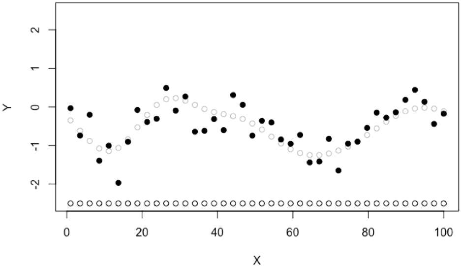
We start by describing the perspective of CRN we take. In the classical non-CRN setting, an optimisation algorithm collects data \((x,y)\) (in black) and predicts the average \(\mathbb{E}[\theta(x)]\) (grey);
.
.
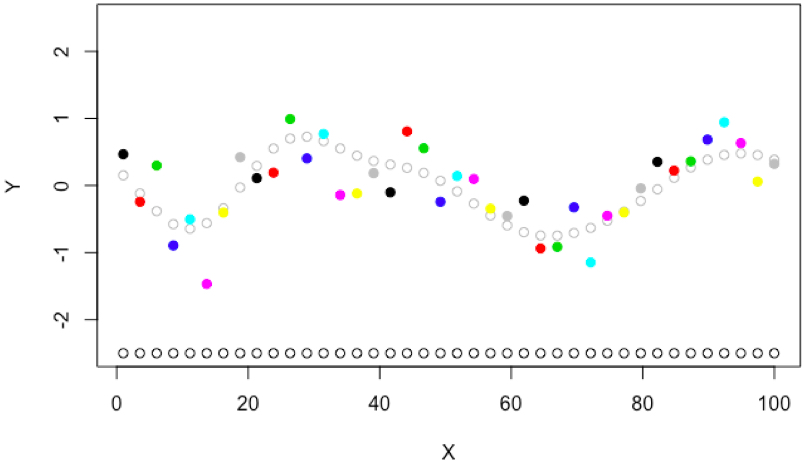
In reality, the stochastic black box \(\theta(x)\) is often a computer program e.g. training of a neural network with random training-valiadation partitions, executing a simulator with randomly generated scenarios, or measuring reward for an agent in a random environment. The stochasticity comes from random number generation within the function. So we may make this explicit \(\theta(x,s)\) where \(s\) is the random number generator seed that controls all stochasticity inside the function. Therefore, the data collected is actually \((x,s,y)\) triplets where the seed \(s\) may be unique for each data point. Coloring data points by seed might look like
.
.
The question naturally arises, what would happen if we repeatedly call the objective function with only a few seeds. By using the same seed for two values \(x_1, x_2\), we say they are evaluated with common random numbers (CRN). For example, some objective functions may produce data that looks like each seed has some structure in it’s noise;
.
.
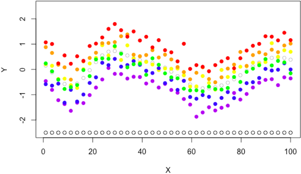
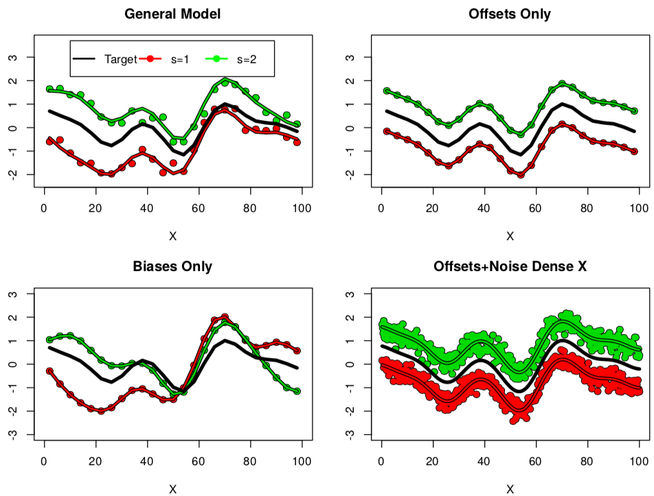
Or in the best possible case, some applications may produce data where a single seed is exactly the same as the average (grey empty points) only with a constant offset, for example the random number stream defines a scenario in a simulator that is easy to solve and outputs at all \(x\) values are increased for seed \(s=1\) (red), or maybe \(s=2\) (purple) leads to scenarios that are hard and all outputs decrease,
.
.
Then the second question naturally arises, in the final case pictured above, surely it is possible to optimise \(\theta(x,1)\) (red) and find \(argmax_x \theta(x,1)\) since this is the same as \(argmax_x\mathbb{E}[\theta(x,\cdot)]\) (grey). Presumably, optimising the deterministic red function above is much easier than optimising the stochastic black function at the very begining of the post! In other words, fixing the seed leads to emergent structure in the noise of a function that can be exploited if it exists.
The Model
The standard approach to global optimisation, places a Gaussian process prior over the underlying average output \(\bar{\theta}(x)=\mathbb{E}[\theta(x,\cdot)]\) which we call the target. We assume that \(\bar{\theta}(x)\) is one sample from a distribution over functions. Then, given \(x\), we assume \(y\) values are the underlying function with added Gaussian noise \(y = \bar{\theta}(x)+\epsilon\), specifically the noise \(\epsilon\) is a Gaussian variable realisation.
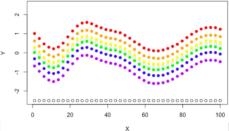
We augment the standard approach by considering a differnt form of noise \(y = \bar{\theta}(x)+\epsilon_s(x)\) where \(\epsilon_{s}(x)\) is a Gaussian process realisation and we call them difference functions because \(\epsilon_s(x) = \theta(x,s) - \bar{\theta}(x)\). These difference functions show how one seed differs from the average over seeds. Since there are (in theory) infintely many possible seeds, there are equally many difference functions, and we require a distribution over difference functions, or, another Gaussian process. In general we model the underlying average (black) with one GP, and all differences (red, green) as samples from another common GP,
.
.
The common GP for the difference functions is a sum of a white noise realisation (top left and bottom right), a constant offset (top right), a bias function (bottom left). In applications where the noise structure is mostly offset (top right), then we can optimise a single seed because \(argmax_x \theta(x,1) \approx argmax_x \bar{\theta}(x)\), in applications where the influence of bias functions and white noise are large, we would need to collect data over lots of seeds to learn \(argmax_x \bar{\theta}(x)\). Mathematically, we may simply dictate that all data collected is over positive seeds, and we may use the model for the unobservable seed \(s=0\) as a prediction of \(\bar{\theta}(x)\)!
The Acquisition Function
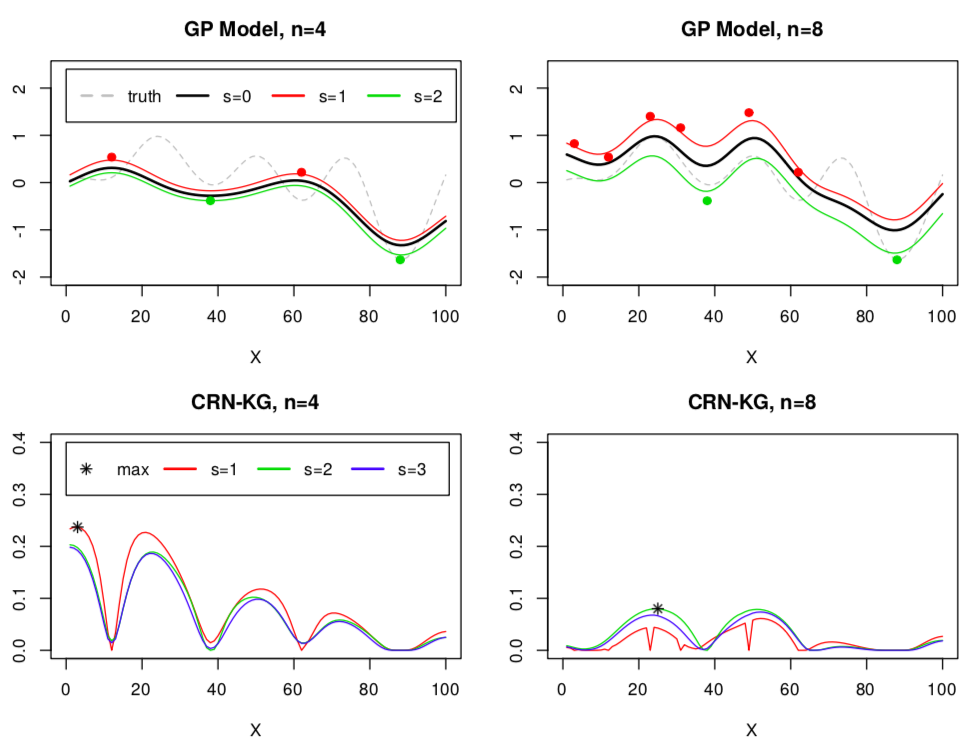
The Knowledge Gradient (KG) acquisition function is a noise generalised variant of the popular Expected Improvement (EI) function, and naturally extends to this use case. We collect data triplets \((x, s, \theta(x,s))\) and we aim to predict \(\bar{\theta}(x)\) and find its peak. Knowledge Gradient is easily adapted to collect data over one domain (inputs \(x\) and positive seeds \(s>0\)) in order to maximise a Gaussian proces over a different domain (inputs \(x\) and seed \(s=0\)). This is achieved by exploiting the correlation structure that is built into the Gaussian process model. This \(KG^{CRN}(x,s)\) acquisition function is maximised over the space of inputs with observed seeds and only a single new seed, to find the next arguments to the objective to be evaluated. For example, starting with 4 points on 2 seeds and sequentially sampling, we see that the next 4 points were naturally allocated to seed \(s=1\) (red),
.
.
The model and acquisition function together define the Knowledge Gradient for Common Random Numbers (CRN-KG) algorithm.
Experiments
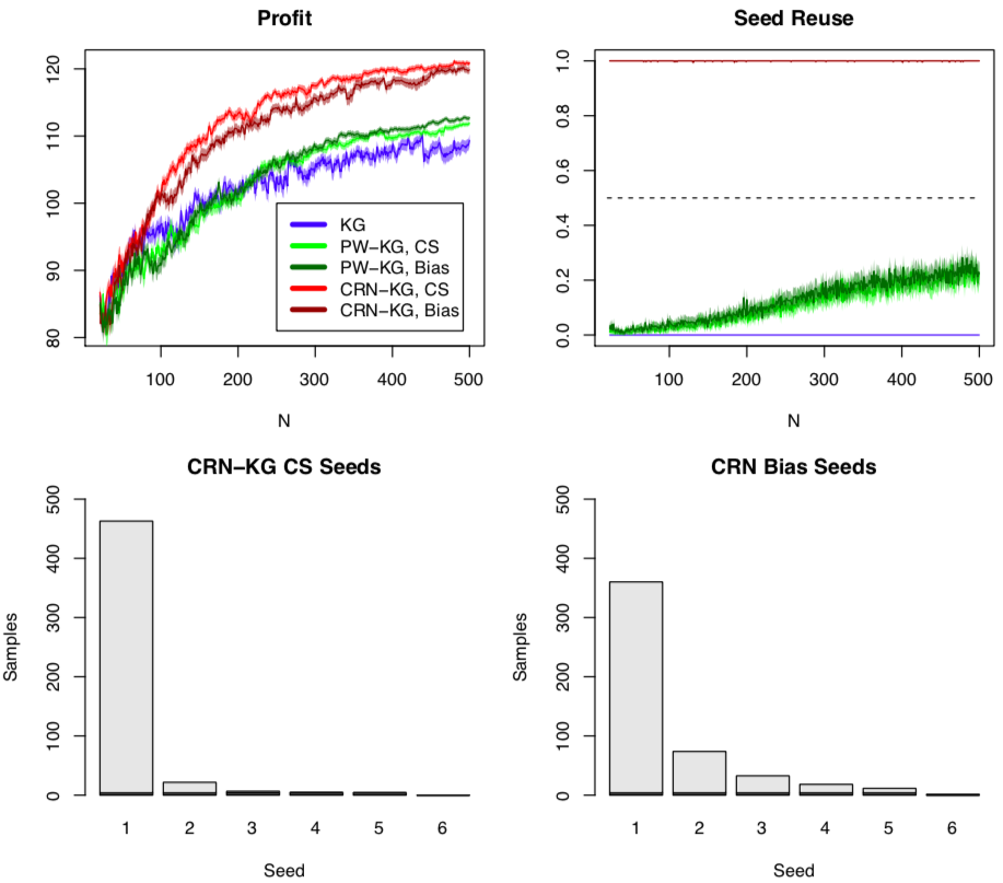
We compare against the standard Knowledge Gradient (all \((x,y)\) pairs have a unique seed) and the Knowledge Gradient with pairwise sampling (PW-KG) designed for the same BO with CRN setting . We apply the algorithm to two simulation optimisation problems, optimising shop restocking levels where the random number seed defines a stream of customers. The goal is to maximise profit. Of all algortihm variants, CRN-KG results in fewer seeds being used, and fewer function calls to convergence. Optimising one single realisation of customer stream leads to a very good optimum of the average over many random customer streams \(\bar{\theta}(x)\).
.
.
The seed reuse shows how frequently a seed sampled at a given iteration, \(s^n\), was in the history of seeds sampled before that iteration \(\{ s^1,...,s^{n-1}\}\). A seed reuse of 1 at iteration \(n\) means that averaged of repeated runs, for that iteration an algorithm always went back to an old seed. The CRN-KG variants never sample a new seed after the initial 5 seeds in this application.
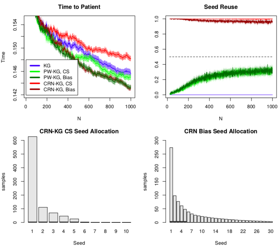
The second application we consider is optimising ambulance base locations on a map to serve patients where the random number seed defines a stream of patients across the map. Contrasting with the previous application, optimising one particular patient realisation does not help optimise the infinite average over seeds,
.
.
Compared to KG for standard global optmisation with identical algortihm setings and implementation, the CRN-KG algorithm has approximltely 10%-20% more computational overhead than standard KG due to two more Gaussian process hyperparameters however acquisition function optimisation is almost the same (PW-KG with identical settings took upto 100% more overhead). And yet exploiting CRN can yield much improved convergence.
For more details, please see the paper!